This function applies generalized additive models (GAM) to assess emerging status for a certain time window.
Usage
apply_gam(
  df,
  y_var,
  eval_years,
  year = "year",
  taxonKey = "taxonKey",
  type_indicator = "observations",
  baseline_var = NULL,
  p_max = 0.1,
  taxon_key = NULL,
  name = NULL,
  df_title = NULL,
  x_label = "year",
  y_label = "Observations",
  saveplot = FALSE,
  dir_name = NULL,
  width = NULL,
  height = NULL,
  verbose = FALSE,
  status_warning = TRUE
)
Arguments
- df
df. A dataframe containing temporal data.
- y_var
character. Name of column containing variable to model. It has to be passed as string, e.g.
"occurrences".- eval_years
numeric. Temporal value(s) when emerging status has to be evaluated.
- year
character. Name of column containing temporal values. It has to be passed as string, e.g.
"time". Default:"year".- taxonKey
character. Name of column containing taxon IDs. It has to be passed as string, e.g.
"taxon". Default:"taxonKey".- type_indicator
character. One of
"observations","occupancy". Used in title of the output plot. Default:"observations".- baseline_var
character. Name of the column containing values to use as additional covariate. Such covariate is introduced in the model to correct research effort bias. Default:
NULL. IfNULLinternal variablemethod_em = "basic", otherwisemethod_em = "correct_baseline". Value ofmethod_emwill be part of title of output plot.- p_max
numeric. A value between 0 and 1. Default: 0.1.
- taxon_key
numeric, character. Taxon key the timeseries belongs to. Used exclusively in graph title and filename (if
saveplot = TRUE). Default:NULL.- name
character. Species name the timeseries belongs to. Used exclusively in graph title and filename (if
saveplot = TRUE). Default:NULL.- df_title
character. Any string you would like to add to graph titles and filenames (if
saveplot = TRUE). The title is always composed of:"GAM"+type_indicator+method_em+taxon_key+name+df_titleseparated by underscore ("_"). Default:NULL.- x_label
character. x-axis label of output plot. Default:
"year".- y_label
character. y-axis label of output plot. Default:
"number of observations".- saveplot
logical. If
TRUEthe plots are automatically saved. Default:FALSE.- dir_name
character. Path of directory where saving plots. If path doesn't exists, directory will be created. Example: "./output/graphs/". If
NULLandsaveplotisTRUE, plots are saved in current directory. Default:NULL.- width
numeric. Plot width in pixels. Values are passed to ggsave. Ignored if
saveplot=FALSE. IfNULLandsaveplotisTRUE,widthis set to 1680 and a message is returned. Default:NULL.- height
numeric. Plot height in pixels. Values are passed to ggsave. Ignored if
saveplot=FALSE. IfNULLandsaveplotisTRUE,heightto 1200 and a message is returned. Default:NULL.- verbose
logical. If
TRUEstatus of processing and possible issues are returned. Default:FALSE.- status_warning
logical. If
TRUEa warning message is added to the plot as textual annotation if the status could not be assessed by GAM. Default:TRUE.
Value
list with six slots:
em_summary: df. A data.frame summarizing the emerging status outputs.em_summarycontains as many rows as the length of input variableeval_year. So, if you evaluate GAM on three years,em_summarywill contain three rows. It contains the following columns:"taxonKey": column containing taxon ID. Column name equal to value of argumenttaxonKey."year": column containing temporal values. Column name equal to value of argumentyear. Column itself is equal to value of argumenteval_years. So, if you evaluate GAM on years 2017, 2018 (eval_years = c(2017, 2018)), you will get these two values in this column.em_status: numeric. Emerging statuses, an integer between 0 and 3.growth: numeric. Lower limit of GAM confidence interval for the first derivative, if positive. It represents the lower guaranteed growth.method: character. GAM method, One of:"correct_baseline"and"basic". See details above in description of argumentuse_baseline.
model: gam object. The model as returned bygam()function.NULLif GAM cannot be applied.output: df. Complete data.frame containing more details than the summaryem_summary. It contains the following columns:all columns in
df.method: character. GAM method, One of:"correct_baseline"and"basic". See details above in description of argumentuse_baseline.fit: numeric. Fit values.ucl: numeric. The upper confidence level values.lcl: numeric. The lower confidence level values.em1: numeric. The emergency value for the 1st derivative. -1, 0 or +1.em2: numeric. The emergency value for the 2nd derivative: -1, 0 or +1.em: numeric. The emergency value: from -4 to +4, based onem1andem2. See Details.em_status: numeric. Emerging statuses, an integer between 0 and 3. See Details.growth: numeric. Lower limit of GAM confidence interval for the first derivative, if positive. It represents the lower guaranteed growth.
first_derivative: df. Data.frame with details of first derivatives. It contains the following columns:smooth: smooth identifier. Example:s(year).derivative: numeric. Value of first derivative.se: numeric. Standard error ofderivative.crit: numeric. Critical value required such thatderivative + (se * crit)andderivative - (se * crit)form the upper and lower bounds of the confidence interval on the first derivative of the estimated smooth at the specific confidence level. In our case the confidence level is hard-coded: 0.8. Thencrit <- qnorm(p = (1-0.8)/2, mean = 0, sd = 1, lower.tail = FALSE).lower_ci: numeric. Lower bound of the confidence interval of the estimated smooth.upper_ci: numeric. Upper bound of the confidence interval of the estimated smooth.value of argument
year: column with temporal values.value of argument
baseline_var: column with the fitted values for the baseline. Ifbaseline_varisNULL, this column is not present.
second_derivative: df. Data.frame with details of second derivatives. Same columns asfirst_derivatives.plot: a ggplot2 object. Plot of observations with GAM output and emerging status. If emerging status cannot be assessed only observations are plotted.
Details
The GAM modelling is performed using the mgcvb::gam(). To use this
function, we pass:
a formula
a family object specifying the distribution
a smoothing parameter estimation method
For more information about all other arguments, see
[mgcv::gam()].If no covariate is used (
baseline_var= NULL), the GAM formula is:n ~ s(year, k = maxk, m = 3, bs = "tp"). Otherwise the GAM formula has a second term,s(n_covariate)and so the GAM formula isn ~ s(year, k = maxk, m = 3, bs = "tp") + s(n_covariate).Description of the parameters present in the formula above:
k: dimension of the basis used to represent the smooth term, i.e. the number of knots used for calculating the smoother. We #' setktomaxk, which is the number of decades in the time series. If less than 5 decades are present in the data,maxkis #' set to 5.bsindicates the basis to use for the smoothing: we uses the default penalized thin plate regression splines.mspecifies the order of the derivatives in the thin plate spline penalty. We usem = 3, the default value.We use
[mgcv::nb()], a negative binomial family to perform the GAM.The smoothing parameter estimation method is set to REML (Restricted maximum likelihood approach). If the P-value of the GAM smoother(s) is/are above threshold value
p_max, GAM is not performed and the next warning is returned: "GAM output cannot be used: p-values of all GAM smoothers are above {p_max}" wherep_maxis the P-value used as threshold as defined by argumentp_max.If the
mgcv::gam()returns an error or a warning, the following message is returned to the user: "GAM ({method_em}) cannot be performed or cannot converge.", wheremethod_emis one of"basic"or"correct_baseline". See argumentbaseline_var.The first and second derivatives of the smoother is calculated using function
gratia::derivatives()with the following hard coded arguments:type: the type of finite difference used. Set to"central".order: 1 for the first derivative, 2 for the second derivativelevel: the confidence level. Set to 0.8eps: the finite difference. Set to 1e-4.For more details, please check derivatives.
The sign of the lower and upper confidence levels of the first and second derivatives are used to define a detailed emergency status (
em) which is internally used to return the emergency status,em_status, which is a column of the returned data.frameem_summary.ucl-1 lcl-1 ucl-2 lcl-2 em em_status + + + + 4 3 (emerging) + + + - 3 3 (emerging) + + - - 2 2 (potentially emerging) - + + + 1 2 (potentially emerging) + - + - 0 1 (unclear) + - - - -1 0 (not emerging) - - + + -2 0 (not emerging) - - + - -3 0 (not emerging) - - - - -4 0 (not emerging)
See also
Other occurrence functions:
apply_decision_rules()
Examples
library(dplyr)
#>
#> Attaching package: ‘dplyr’
#> The following objects are masked from ‘package:stats’:
#>
#> filter, lag
#> The following objects are masked from ‘package:base’:
#>
#> intersect, setdiff, setequal, union
df_gam <- tibble(
taxonKey = rep(3003709, 24),
canonicalName = rep("Rosa glauca", 24),
year = seq(1995, 2018),
n = c(
1, 1, 0, 0, 0, 2, 0, 0, 1, 3, 1, 2, 0, 5, 0, 5, 4, 2, 1,
1, 3, 3, 8, 10
),
n_class = c(
229, 555, 1116, 939, 919, 853, 442, 532, 623, 1178, 732, 371, 1053,
1001, 1550, 1142, 1076, 1310, 922, 1773, 1637,
1866, 2234, 2013
)
)
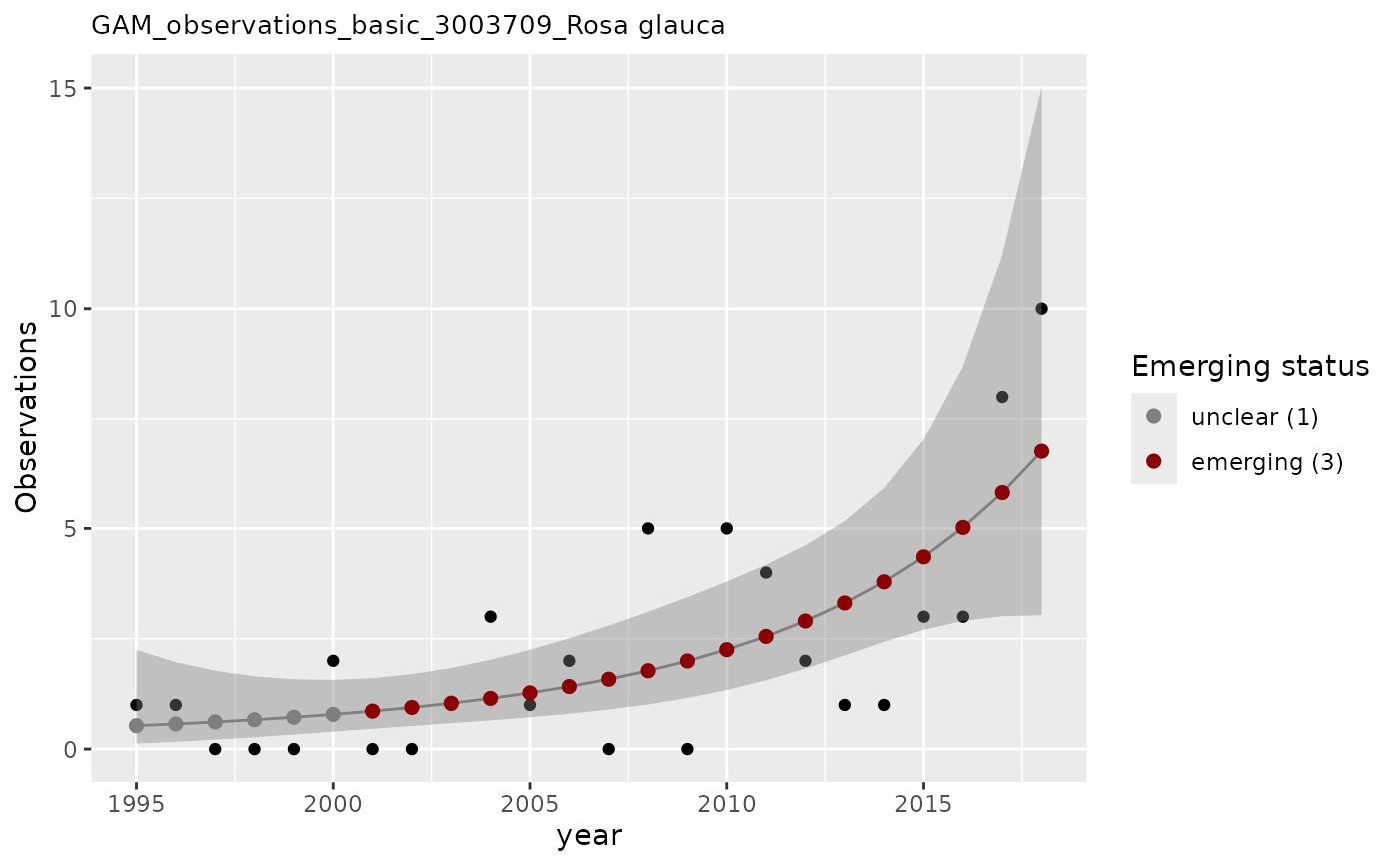
# apply GAM to n without baseline as covariate
apply_gam(df_gam,
y_var = "n",
eval_years = 2018,
taxon_key = 3003709,
name = "Rosa glauca",
verbose = TRUE
)
#> [1] "Analyzing: Rosa glauca(3003709)"
#> $em_summary
#> # A tibble: 1 × 5
#> taxonKey year em_status growth method
#> <dbl> <dbl> <dbl> <dbl> <chr>
#> 1 3003709 2018 3 1.02 basic
#>
#> $model
#>
#> Family: Negative Binomial(3.527)
#> Link function: log
#>
#> Formula:
#> n ~ s(year, k = maxk, m = 3, bs = "tp")
#>
#> Estimated degrees of freedom:
#> 2 total = 3
#>
#> REML score: 42.28844
#>
#> $output
#> # A tibble: 24 × 14
#> taxonKey canonicalName year n n_class method fit ucl lcl em1
#> <dbl> <chr> <dbl> <dbl> <dbl> <chr> <dbl> <dbl> <dbl> <dbl>
#> 1 3003709 Rosa glauca 1995 1 229 basic 0.530 2.25 0.125 0
#> 2 3003709 Rosa glauca 1996 1 555 basic 0.570 1.97 0.165 0
#> 3 3003709 Rosa glauca 1997 0 1116 basic 0.614 1.78 0.212 0
#> 4 3003709 Rosa glauca 1998 0 939 basic 0.664 1.65 0.268 0
#> 5 3003709 Rosa glauca 1999 0 919 basic 0.721 1.58 0.329 0
#> 6 3003709 Rosa glauca 2000 2 853 basic 0.786 1.57 0.394 0
#> 7 3003709 Rosa glauca 2001 0 442 basic 0.859 1.61 0.460 0
#> 8 3003709 Rosa glauca 2002 0 532 basic 0.943 1.70 0.524 1
#> 9 3003709 Rosa glauca 2003 1 623 basic 1.04 1.84 0.587 1
#> 10 3003709 Rosa glauca 2004 3 1178 basic 1.15 2.02 0.651 1
#> # ℹ 14 more rows
#> # ℹ 4 more variables: em2 <dbl>, em <dbl>, em_status <dbl>, growth <dbl>
#>
#> $first_derivative
#> # A tibble: 24 × 7
#> smooth derivative se crit lower_ci upper_ci year
#> <chr> <dbl> <dbl> <dbl> <dbl> <dbl> <dbl>
#> 1 s(year) 0.0699 0.124 1.28 -0.0891 0.229 1995.
#> 2 s(year) 0.0734 0.115 1.28 -0.0739 0.221 1996.
#> 3 s(year) 0.0770 0.106 1.28 -0.0588 0.213 1997.
#> 4 s(year) 0.0805 0.0970 1.28 -0.0437 0.205 1998.
#> 5 s(year) 0.0841 0.0881 1.28 -0.0288 0.197 1999.
#> 6 s(year) 0.0876 0.0793 1.28 -0.0140 0.189 2000.
#> 7 s(year) 0.0911 0.0707 1.28 0.000581 0.182 2001.
#> 8 s(year) 0.0947 0.0623 1.28 0.0149 0.174 2002.
#> 9 s(year) 0.0982 0.0542 1.28 0.0288 0.168 2003.
#> 10 s(year) 0.102 0.0466 1.28 0.0421 0.161 2004.
#> # ℹ 14 more rows
#>
#> $second_derivative
#> # A tibble: 24 × 7
#> smooth derivative se crit lower_ci upper_ci year
#> <chr> <dbl> <dbl> <dbl> <dbl> <dbl> <dbl>
#> 1 s(year) 0.00354 0.00938 1.28 -0.00847 0.0156 1995.
#> 2 s(year) 0.00354 0.00938 1.28 -0.00847 0.0156 1996.
#> 3 s(year) 0.00354 0.00937 1.28 -0.00847 0.0156 1997.
#> 4 s(year) 0.00354 0.00937 1.28 -0.00847 0.0156 1998.
#> 5 s(year) 0.00354 0.00937 1.28 -0.00847 0.0156 1999.
#> 6 s(year) 0.00354 0.00937 1.28 -0.00847 0.0156 2000.
#> 7 s(year) 0.00354 0.00937 1.28 -0.00847 0.0156 2001.
#> 8 s(year) 0.00354 0.00937 1.28 -0.00847 0.0156 2002.
#> 9 s(year) 0.00354 0.00937 1.28 -0.00847 0.0156 2003.
#> 10 s(year) 0.00354 0.00937 1.28 -0.00847 0.0156 2004.
#> # ℹ 14 more rows
#>
#> $plot
 #>
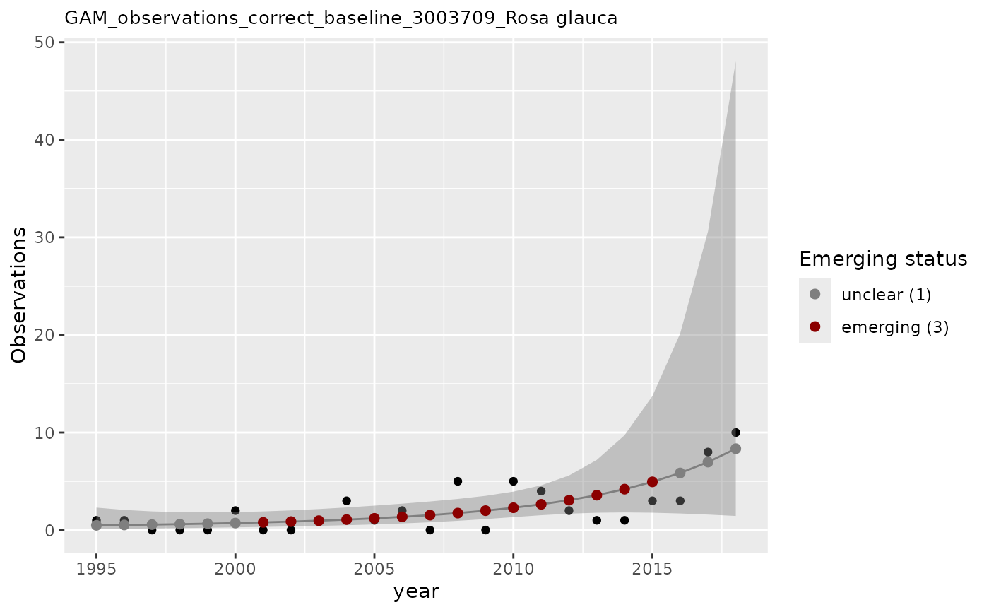
# apply GAM using baseline data in column n_class as covariate
apply_gam(df_gam,
y_var = "n",
eval_years = 2018,
baseline_var = "n_class",
taxon_key = 3003709,
name = "Rosa glauca",
verbose = TRUE
)
#> [1] "Analyzing: Rosa glauca(3003709)"
#> $em_summary
#> # A tibble: 1 × 5
#> taxonKey year em_status growth method
#> <dbl> <dbl> <dbl> <dbl> <chr>
#> 1 3003709 2018 1 0.980 correct_baseline
#>
#> $model
#>
#> Family: Negative Binomial(2.907)
#> Link function: log
#>
#> Formula:
#> n ~ s(year, k = maxk, m = 3, bs = "tp") + s(n_class)
#>
#> Estimated degrees of freedom:
#> 2 1 total = 4
#>
#> REML score: 42.23685
#>
#> $output
#> # A tibble: 24 × 14
#> taxonKey canonicalName year n n_class method fit ucl lcl em1
#> <dbl> <chr> <dbl> <dbl> <dbl> <chr> <dbl> <dbl> <dbl> <dbl>
#> 1 3003709 Rosa glauca 1995 1 229 correct_b… 0.488 2.30 0.103 0
#> 2 3003709 Rosa glauca 1996 1 555 correct_b… 0.522 2.07 0.132 0
#> 3 3003709 Rosa glauca 1997 0 1116 correct_b… 0.561 1.92 0.164 0
#> 4 3003709 Rosa glauca 1998 0 939 correct_b… 0.606 1.84 0.200 0
#> 5 3003709 Rosa glauca 1999 0 919 correct_b… 0.658 1.82 0.239 0
#> 6 3003709 Rosa glauca 2000 2 853 correct_b… 0.719 1.84 0.280 0
#> 7 3003709 Rosa glauca 2001 0 442 correct_b… 0.789 1.91 0.325 0
#> 8 3003709 Rosa glauca 2002 0 532 correct_b… 0.870 2.02 0.375 1
#> 9 3003709 Rosa glauca 2003 1 623 correct_b… 0.964 2.16 0.431 1
#> 10 3003709 Rosa glauca 2004 3 1178 correct_b… 1.07 2.32 0.498 1
#> # ℹ 14 more rows
#> # ℹ 4 more variables: em2 <dbl>, em <dbl>, em_status <dbl>, growth <dbl>
#>
#> $first_derivative
#> # A tibble: 48 × 8
#> smooth derivative se crit lower_ci upper_ci year n_class
#> <chr> <dbl> <dbl> <dbl> <dbl> <dbl> <dbl> <dbl>
#> 1 s(year) 0.0647 0.131 1.28 -0.103 0.232 1995. NA
#> 2 s(year) 0.0698 0.120 1.28 -0.0840 0.224 1996. NA
#> 3 s(year) 0.0749 0.110 1.28 -0.0657 0.216 1997. NA
#> 4 s(year) 0.0800 0.0998 1.28 -0.0479 0.208 1998. NA
#> 5 s(year) 0.0851 0.0902 1.28 -0.0305 0.201 1999. NA
#> 6 s(year) 0.0902 0.0812 1.28 -0.0138 0.194 2000. NA
#> 7 s(year) 0.0953 0.0728 1.28 0.00198 0.189 2001. NA
#> 8 s(year) 0.100 0.0656 1.28 0.0164 0.184 2002. NA
#> 9 s(year) 0.106 0.0597 1.28 0.0291 0.182 2003. NA
#> 10 s(year) 0.111 0.0556 1.28 0.0394 0.182 2004. NA
#> # ℹ 38 more rows
#>
#> $second_derivative
#> # A tibble: 48 × 8
#> smooth derivative se crit lower_ci upper_ci year n_class
#> <chr> <dbl> <dbl> <dbl> <dbl> <dbl> <dbl> <dbl>
#> 1 s(year) 0.00511 0.0116 1.28 -0.00979 0.0200 1995. NA
#> 2 s(year) 0.00511 0.0116 1.28 -0.00979 0.0200 1996. NA
#> 3 s(year) 0.00511 0.0116 1.28 -0.00979 0.0200 1997. NA
#> 4 s(year) 0.00511 0.0116 1.28 -0.00979 0.0200 1998. NA
#> 5 s(year) 0.00511 0.0116 1.28 -0.00979 0.0200 1999. NA
#> 6 s(year) 0.00511 0.0116 1.28 -0.00979 0.0200 2000. NA
#> 7 s(year) 0.00511 0.0116 1.28 -0.00979 0.0200 2001. NA
#> 8 s(year) 0.00511 0.0116 1.28 -0.00979 0.0200 2002. NA
#> 9 s(year) 0.00511 0.0116 1.28 -0.00979 0.0200 2003. NA
#> 10 s(year) 0.00511 0.0116 1.28 -0.00979 0.0200 2004. NA
#> # ℹ 38 more rows
#>
#> $plot
#>
# apply GAM using baseline data in column n_class as covariate
apply_gam(df_gam,
y_var = "n",
eval_years = 2018,
baseline_var = "n_class",
taxon_key = 3003709,
name = "Rosa glauca",
verbose = TRUE
)
#> [1] "Analyzing: Rosa glauca(3003709)"
#> $em_summary
#> # A tibble: 1 × 5
#> taxonKey year em_status growth method
#> <dbl> <dbl> <dbl> <dbl> <chr>
#> 1 3003709 2018 1 0.980 correct_baseline
#>
#> $model
#>
#> Family: Negative Binomial(2.907)
#> Link function: log
#>
#> Formula:
#> n ~ s(year, k = maxk, m = 3, bs = "tp") + s(n_class)
#>
#> Estimated degrees of freedom:
#> 2 1 total = 4
#>
#> REML score: 42.23685
#>
#> $output
#> # A tibble: 24 × 14
#> taxonKey canonicalName year n n_class method fit ucl lcl em1
#> <dbl> <chr> <dbl> <dbl> <dbl> <chr> <dbl> <dbl> <dbl> <dbl>
#> 1 3003709 Rosa glauca 1995 1 229 correct_b… 0.488 2.30 0.103 0
#> 2 3003709 Rosa glauca 1996 1 555 correct_b… 0.522 2.07 0.132 0
#> 3 3003709 Rosa glauca 1997 0 1116 correct_b… 0.561 1.92 0.164 0
#> 4 3003709 Rosa glauca 1998 0 939 correct_b… 0.606 1.84 0.200 0
#> 5 3003709 Rosa glauca 1999 0 919 correct_b… 0.658 1.82 0.239 0
#> 6 3003709 Rosa glauca 2000 2 853 correct_b… 0.719 1.84 0.280 0
#> 7 3003709 Rosa glauca 2001 0 442 correct_b… 0.789 1.91 0.325 0
#> 8 3003709 Rosa glauca 2002 0 532 correct_b… 0.870 2.02 0.375 1
#> 9 3003709 Rosa glauca 2003 1 623 correct_b… 0.964 2.16 0.431 1
#> 10 3003709 Rosa glauca 2004 3 1178 correct_b… 1.07 2.32 0.498 1
#> # ℹ 14 more rows
#> # ℹ 4 more variables: em2 <dbl>, em <dbl>, em_status <dbl>, growth <dbl>
#>
#> $first_derivative
#> # A tibble: 48 × 8
#> smooth derivative se crit lower_ci upper_ci year n_class
#> <chr> <dbl> <dbl> <dbl> <dbl> <dbl> <dbl> <dbl>
#> 1 s(year) 0.0647 0.131 1.28 -0.103 0.232 1995. NA
#> 2 s(year) 0.0698 0.120 1.28 -0.0840 0.224 1996. NA
#> 3 s(year) 0.0749 0.110 1.28 -0.0657 0.216 1997. NA
#> 4 s(year) 0.0800 0.0998 1.28 -0.0479 0.208 1998. NA
#> 5 s(year) 0.0851 0.0902 1.28 -0.0305 0.201 1999. NA
#> 6 s(year) 0.0902 0.0812 1.28 -0.0138 0.194 2000. NA
#> 7 s(year) 0.0953 0.0728 1.28 0.00198 0.189 2001. NA
#> 8 s(year) 0.100 0.0656 1.28 0.0164 0.184 2002. NA
#> 9 s(year) 0.106 0.0597 1.28 0.0291 0.182 2003. NA
#> 10 s(year) 0.111 0.0556 1.28 0.0394 0.182 2004. NA
#> # ℹ 38 more rows
#>
#> $second_derivative
#> # A tibble: 48 × 8
#> smooth derivative se crit lower_ci upper_ci year n_class
#> <chr> <dbl> <dbl> <dbl> <dbl> <dbl> <dbl> <dbl>
#> 1 s(year) 0.00511 0.0116 1.28 -0.00979 0.0200 1995. NA
#> 2 s(year) 0.00511 0.0116 1.28 -0.00979 0.0200 1996. NA
#> 3 s(year) 0.00511 0.0116 1.28 -0.00979 0.0200 1997. NA
#> 4 s(year) 0.00511 0.0116 1.28 -0.00979 0.0200 1998. NA
#> 5 s(year) 0.00511 0.0116 1.28 -0.00979 0.0200 1999. NA
#> 6 s(year) 0.00511 0.0116 1.28 -0.00979 0.0200 2000. NA
#> 7 s(year) 0.00511 0.0116 1.28 -0.00979 0.0200 2001. NA
#> 8 s(year) 0.00511 0.0116 1.28 -0.00979 0.0200 2002. NA
#> 9 s(year) 0.00511 0.0116 1.28 -0.00979 0.0200 2003. NA
#> 10 s(year) 0.00511 0.0116 1.28 -0.00979 0.0200 2004. NA
#> # ℹ 38 more rows
#>
#> $plot
 #>
# apply GAM using n as occupancy values, evaluate on two years. No baseline
apply_gam(df_gam,
y_var = "n",
eval_years = c(2017, 2018),
taxon_key = 3003709,
type_indicator = "occupancy",
name = "Rosa glauca",
y_label = "measured occupancy",
verbose = TRUE
)
#> [1] "Analyzing: Rosa glauca(3003709)"
#> $em_summary
#> # A tibble: 2 × 5
#> taxonKey year em_status growth method
#> <dbl> <dbl> <dbl> <dbl> <chr>
#> 1 3003709 2017 3 1.03 basic
#> 2 3003709 2018 3 1.02 basic
#>
#> $model
#>
#> Family: Negative Binomial(3.527)
#> Link function: log
#>
#> Formula:
#> n ~ s(year, k = maxk, m = 3, bs = "tp")
#>
#> Estimated degrees of freedom:
#> 2 total = 3
#>
#> REML score: 42.28844
#>
#> $output
#> # A tibble: 24 × 14
#> taxonKey canonicalName year n n_class method fit ucl lcl em1
#> <dbl> <chr> <dbl> <dbl> <dbl> <chr> <dbl> <dbl> <dbl> <dbl>
#> 1 3003709 Rosa glauca 1995 1 229 basic 0.530 2.25 0.125 0
#> 2 3003709 Rosa glauca 1996 1 555 basic 0.570 1.97 0.165 0
#> 3 3003709 Rosa glauca 1997 0 1116 basic 0.614 1.78 0.212 0
#> 4 3003709 Rosa glauca 1998 0 939 basic 0.664 1.65 0.268 0
#> 5 3003709 Rosa glauca 1999 0 919 basic 0.721 1.58 0.329 0
#> 6 3003709 Rosa glauca 2000 2 853 basic 0.786 1.57 0.394 0
#> 7 3003709 Rosa glauca 2001 0 442 basic 0.859 1.61 0.460 0
#> 8 3003709 Rosa glauca 2002 0 532 basic 0.943 1.70 0.524 1
#> 9 3003709 Rosa glauca 2003 1 623 basic 1.04 1.84 0.587 1
#> 10 3003709 Rosa glauca 2004 3 1178 basic 1.15 2.02 0.651 1
#> # ℹ 14 more rows
#> # ℹ 4 more variables: em2 <dbl>, em <dbl>, em_status <dbl>, growth <dbl>
#>
#> $first_derivative
#> # A tibble: 24 × 7
#> smooth derivative se crit lower_ci upper_ci year
#> <chr> <dbl> <dbl> <dbl> <dbl> <dbl> <dbl>
#> 1 s(year) 0.0699 0.124 1.28 -0.0891 0.229 1995.
#> 2 s(year) 0.0734 0.115 1.28 -0.0739 0.221 1996.
#> 3 s(year) 0.0770 0.106 1.28 -0.0588 0.213 1997.
#> 4 s(year) 0.0805 0.0970 1.28 -0.0437 0.205 1998.
#> 5 s(year) 0.0841 0.0881 1.28 -0.0288 0.197 1999.
#> 6 s(year) 0.0876 0.0793 1.28 -0.0140 0.189 2000.
#> 7 s(year) 0.0911 0.0707 1.28 0.000581 0.182 2001.
#> 8 s(year) 0.0947 0.0623 1.28 0.0149 0.174 2002.
#> 9 s(year) 0.0982 0.0542 1.28 0.0288 0.168 2003.
#> 10 s(year) 0.102 0.0466 1.28 0.0421 0.161 2004.
#> # ℹ 14 more rows
#>
#> $second_derivative
#> # A tibble: 24 × 7
#> smooth derivative se crit lower_ci upper_ci year
#> <chr> <dbl> <dbl> <dbl> <dbl> <dbl> <dbl>
#> 1 s(year) 0.00354 0.00938 1.28 -0.00847 0.0156 1995.
#> 2 s(year) 0.00354 0.00938 1.28 -0.00847 0.0156 1996.
#> 3 s(year) 0.00354 0.00937 1.28 -0.00847 0.0156 1997.
#> 4 s(year) 0.00354 0.00937 1.28 -0.00847 0.0156 1998.
#> 5 s(year) 0.00354 0.00937 1.28 -0.00847 0.0156 1999.
#> 6 s(year) 0.00354 0.00937 1.28 -0.00847 0.0156 2000.
#> 7 s(year) 0.00354 0.00937 1.28 -0.00847 0.0156 2001.
#> 8 s(year) 0.00354 0.00937 1.28 -0.00847 0.0156 2002.
#> 9 s(year) 0.00354 0.00937 1.28 -0.00847 0.0156 2003.
#> 10 s(year) 0.00354 0.00937 1.28 -0.00847 0.0156 2004.
#> # ℹ 14 more rows
#>
#> $plot
#>
# apply GAM using n as occupancy values, evaluate on two years. No baseline
apply_gam(df_gam,
y_var = "n",
eval_years = c(2017, 2018),
taxon_key = 3003709,
type_indicator = "occupancy",
name = "Rosa glauca",
y_label = "measured occupancy",
verbose = TRUE
)
#> [1] "Analyzing: Rosa glauca(3003709)"
#> $em_summary
#> # A tibble: 2 × 5
#> taxonKey year em_status growth method
#> <dbl> <dbl> <dbl> <dbl> <chr>
#> 1 3003709 2017 3 1.03 basic
#> 2 3003709 2018 3 1.02 basic
#>
#> $model
#>
#> Family: Negative Binomial(3.527)
#> Link function: log
#>
#> Formula:
#> n ~ s(year, k = maxk, m = 3, bs = "tp")
#>
#> Estimated degrees of freedom:
#> 2 total = 3
#>
#> REML score: 42.28844
#>
#> $output
#> # A tibble: 24 × 14
#> taxonKey canonicalName year n n_class method fit ucl lcl em1
#> <dbl> <chr> <dbl> <dbl> <dbl> <chr> <dbl> <dbl> <dbl> <dbl>
#> 1 3003709 Rosa glauca 1995 1 229 basic 0.530 2.25 0.125 0
#> 2 3003709 Rosa glauca 1996 1 555 basic 0.570 1.97 0.165 0
#> 3 3003709 Rosa glauca 1997 0 1116 basic 0.614 1.78 0.212 0
#> 4 3003709 Rosa glauca 1998 0 939 basic 0.664 1.65 0.268 0
#> 5 3003709 Rosa glauca 1999 0 919 basic 0.721 1.58 0.329 0
#> 6 3003709 Rosa glauca 2000 2 853 basic 0.786 1.57 0.394 0
#> 7 3003709 Rosa glauca 2001 0 442 basic 0.859 1.61 0.460 0
#> 8 3003709 Rosa glauca 2002 0 532 basic 0.943 1.70 0.524 1
#> 9 3003709 Rosa glauca 2003 1 623 basic 1.04 1.84 0.587 1
#> 10 3003709 Rosa glauca 2004 3 1178 basic 1.15 2.02 0.651 1
#> # ℹ 14 more rows
#> # ℹ 4 more variables: em2 <dbl>, em <dbl>, em_status <dbl>, growth <dbl>
#>
#> $first_derivative
#> # A tibble: 24 × 7
#> smooth derivative se crit lower_ci upper_ci year
#> <chr> <dbl> <dbl> <dbl> <dbl> <dbl> <dbl>
#> 1 s(year) 0.0699 0.124 1.28 -0.0891 0.229 1995.
#> 2 s(year) 0.0734 0.115 1.28 -0.0739 0.221 1996.
#> 3 s(year) 0.0770 0.106 1.28 -0.0588 0.213 1997.
#> 4 s(year) 0.0805 0.0970 1.28 -0.0437 0.205 1998.
#> 5 s(year) 0.0841 0.0881 1.28 -0.0288 0.197 1999.
#> 6 s(year) 0.0876 0.0793 1.28 -0.0140 0.189 2000.
#> 7 s(year) 0.0911 0.0707 1.28 0.000581 0.182 2001.
#> 8 s(year) 0.0947 0.0623 1.28 0.0149 0.174 2002.
#> 9 s(year) 0.0982 0.0542 1.28 0.0288 0.168 2003.
#> 10 s(year) 0.102 0.0466 1.28 0.0421 0.161 2004.
#> # ℹ 14 more rows
#>
#> $second_derivative
#> # A tibble: 24 × 7
#> smooth derivative se crit lower_ci upper_ci year
#> <chr> <dbl> <dbl> <dbl> <dbl> <dbl> <dbl>
#> 1 s(year) 0.00354 0.00938 1.28 -0.00847 0.0156 1995.
#> 2 s(year) 0.00354 0.00938 1.28 -0.00847 0.0156 1996.
#> 3 s(year) 0.00354 0.00937 1.28 -0.00847 0.0156 1997.
#> 4 s(year) 0.00354 0.00937 1.28 -0.00847 0.0156 1998.
#> 5 s(year) 0.00354 0.00937 1.28 -0.00847 0.0156 1999.
#> 6 s(year) 0.00354 0.00937 1.28 -0.00847 0.0156 2000.
#> 7 s(year) 0.00354 0.00937 1.28 -0.00847 0.0156 2001.
#> 8 s(year) 0.00354 0.00937 1.28 -0.00847 0.0156 2002.
#> 9 s(year) 0.00354 0.00937 1.28 -0.00847 0.0156 2003.
#> 10 s(year) 0.00354 0.00937 1.28 -0.00847 0.0156 2004.
#> # ℹ 14 more rows
#>
#> $plot
 #>
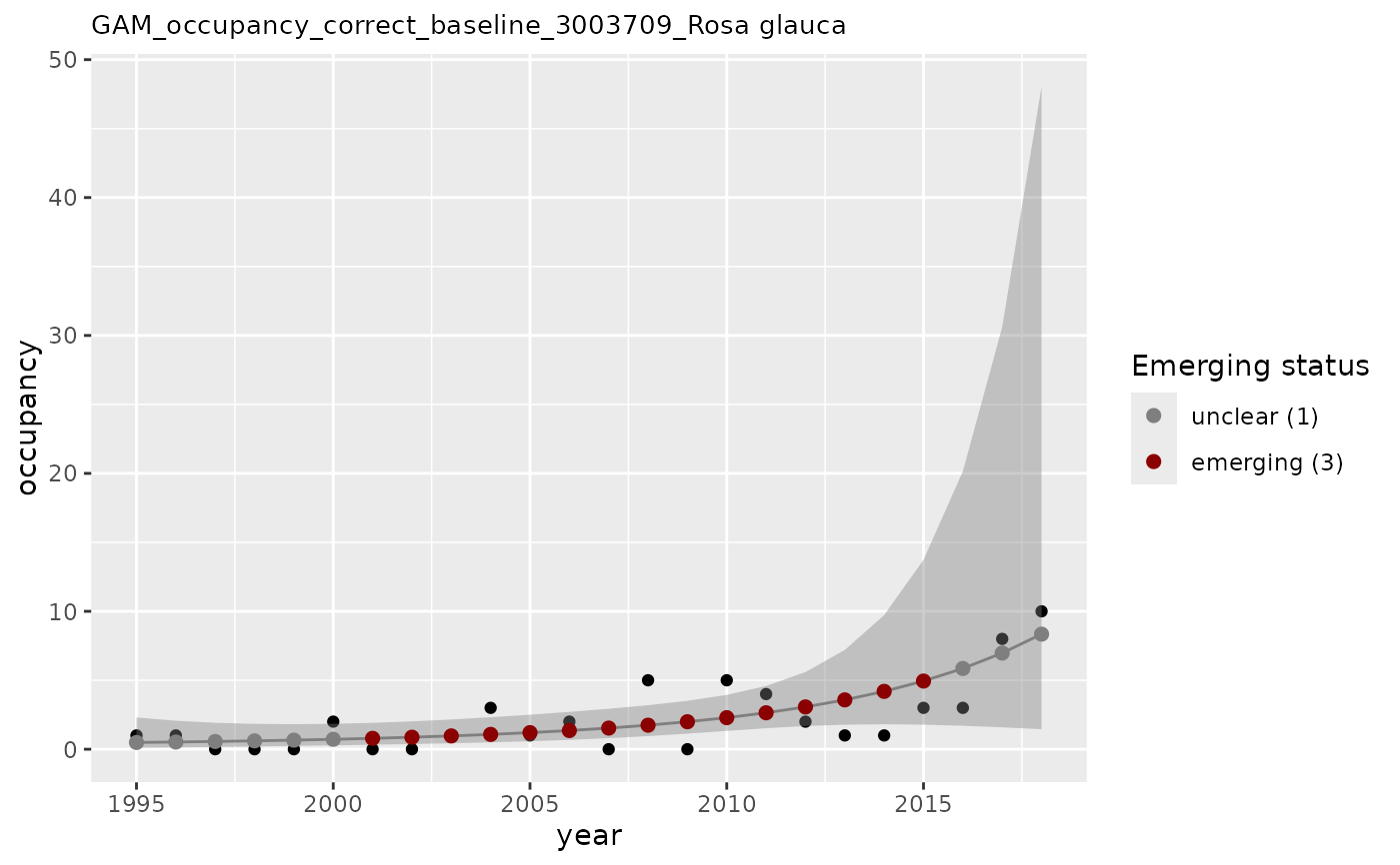
# apply GAM using n as occupancy values and n_class as covariate (baseline)
apply_gam(df_gam,
y_var = "n",
eval_years = c(2017, 2018),
baseline_var = "n_class",
taxon_key = 3003709,
type_indicator = "occupancy",
name = "Rosa glauca",
y_label = "measured occupancy",
verbose = TRUE
)
#> [1] "Analyzing: Rosa glauca(3003709)"
#> $em_summary
#> # A tibble: 2 × 5
#> taxonKey year em_status growth method
#> <dbl> <dbl> <dbl> <dbl> <chr>
#> 1 3003709 2017 1 0.989 correct_baseline
#> 2 3003709 2018 1 0.980 correct_baseline
#>
#> $model
#>
#> Family: Negative Binomial(2.907)
#> Link function: log
#>
#> Formula:
#> n ~ s(year, k = maxk, m = 3, bs = "tp") + s(n_class)
#>
#> Estimated degrees of freedom:
#> 2 1 total = 4
#>
#> REML score: 42.23685
#>
#> $output
#> # A tibble: 24 × 14
#> taxonKey canonicalName year n n_class method fit ucl lcl em1
#> <dbl> <chr> <dbl> <dbl> <dbl> <chr> <dbl> <dbl> <dbl> <dbl>
#> 1 3003709 Rosa glauca 1995 1 229 correct_b… 0.488 2.30 0.103 0
#> 2 3003709 Rosa glauca 1996 1 555 correct_b… 0.522 2.07 0.132 0
#> 3 3003709 Rosa glauca 1997 0 1116 correct_b… 0.561 1.92 0.164 0
#> 4 3003709 Rosa glauca 1998 0 939 correct_b… 0.606 1.84 0.200 0
#> 5 3003709 Rosa glauca 1999 0 919 correct_b… 0.658 1.82 0.239 0
#> 6 3003709 Rosa glauca 2000 2 853 correct_b… 0.719 1.84 0.280 0
#> 7 3003709 Rosa glauca 2001 0 442 correct_b… 0.789 1.91 0.325 0
#> 8 3003709 Rosa glauca 2002 0 532 correct_b… 0.870 2.02 0.375 1
#> 9 3003709 Rosa glauca 2003 1 623 correct_b… 0.964 2.16 0.431 1
#> 10 3003709 Rosa glauca 2004 3 1178 correct_b… 1.07 2.32 0.498 1
#> # ℹ 14 more rows
#> # ℹ 4 more variables: em2 <dbl>, em <dbl>, em_status <dbl>, growth <dbl>
#>
#> $first_derivative
#> # A tibble: 48 × 8
#> smooth derivative se crit lower_ci upper_ci year n_class
#> <chr> <dbl> <dbl> <dbl> <dbl> <dbl> <dbl> <dbl>
#> 1 s(year) 0.0647 0.131 1.28 -0.103 0.232 1995. NA
#> 2 s(year) 0.0698 0.120 1.28 -0.0840 0.224 1996. NA
#> 3 s(year) 0.0749 0.110 1.28 -0.0657 0.216 1997. NA
#> 4 s(year) 0.0800 0.0998 1.28 -0.0479 0.208 1998. NA
#> 5 s(year) 0.0851 0.0902 1.28 -0.0305 0.201 1999. NA
#> 6 s(year) 0.0902 0.0812 1.28 -0.0138 0.194 2000. NA
#> 7 s(year) 0.0953 0.0728 1.28 0.00198 0.189 2001. NA
#> 8 s(year) 0.100 0.0656 1.28 0.0164 0.184 2002. NA
#> 9 s(year) 0.106 0.0597 1.28 0.0291 0.182 2003. NA
#> 10 s(year) 0.111 0.0556 1.28 0.0394 0.182 2004. NA
#> # ℹ 38 more rows
#>
#> $second_derivative
#> # A tibble: 48 × 8
#> smooth derivative se crit lower_ci upper_ci year n_class
#> <chr> <dbl> <dbl> <dbl> <dbl> <dbl> <dbl> <dbl>
#> 1 s(year) 0.00511 0.0116 1.28 -0.00979 0.0200 1995. NA
#> 2 s(year) 0.00511 0.0116 1.28 -0.00979 0.0200 1996. NA
#> 3 s(year) 0.00511 0.0116 1.28 -0.00979 0.0200 1997. NA
#> 4 s(year) 0.00511 0.0116 1.28 -0.00979 0.0200 1998. NA
#> 5 s(year) 0.00511 0.0116 1.28 -0.00979 0.0200 1999. NA
#> 6 s(year) 0.00511 0.0116 1.28 -0.00979 0.0200 2000. NA
#> 7 s(year) 0.00511 0.0116 1.28 -0.00979 0.0200 2001. NA
#> 8 s(year) 0.00511 0.0116 1.28 -0.00979 0.0200 2002. NA
#> 9 s(year) 0.00511 0.0116 1.28 -0.00979 0.0200 2003. NA
#> 10 s(year) 0.00511 0.0116 1.28 -0.00979 0.0200 2004. NA
#> # ℹ 38 more rows
#>
#> $plot
#>
# apply GAM using n as occupancy values and n_class as covariate (baseline)
apply_gam(df_gam,
y_var = "n",
eval_years = c(2017, 2018),
baseline_var = "n_class",
taxon_key = 3003709,
type_indicator = "occupancy",
name = "Rosa glauca",
y_label = "measured occupancy",
verbose = TRUE
)
#> [1] "Analyzing: Rosa glauca(3003709)"
#> $em_summary
#> # A tibble: 2 × 5
#> taxonKey year em_status growth method
#> <dbl> <dbl> <dbl> <dbl> <chr>
#> 1 3003709 2017 1 0.989 correct_baseline
#> 2 3003709 2018 1 0.980 correct_baseline
#>
#> $model
#>
#> Family: Negative Binomial(2.907)
#> Link function: log
#>
#> Formula:
#> n ~ s(year, k = maxk, m = 3, bs = "tp") + s(n_class)
#>
#> Estimated degrees of freedom:
#> 2 1 total = 4
#>
#> REML score: 42.23685
#>
#> $output
#> # A tibble: 24 × 14
#> taxonKey canonicalName year n n_class method fit ucl lcl em1
#> <dbl> <chr> <dbl> <dbl> <dbl> <chr> <dbl> <dbl> <dbl> <dbl>
#> 1 3003709 Rosa glauca 1995 1 229 correct_b… 0.488 2.30 0.103 0
#> 2 3003709 Rosa glauca 1996 1 555 correct_b… 0.522 2.07 0.132 0
#> 3 3003709 Rosa glauca 1997 0 1116 correct_b… 0.561 1.92 0.164 0
#> 4 3003709 Rosa glauca 1998 0 939 correct_b… 0.606 1.84 0.200 0
#> 5 3003709 Rosa glauca 1999 0 919 correct_b… 0.658 1.82 0.239 0
#> 6 3003709 Rosa glauca 2000 2 853 correct_b… 0.719 1.84 0.280 0
#> 7 3003709 Rosa glauca 2001 0 442 correct_b… 0.789 1.91 0.325 0
#> 8 3003709 Rosa glauca 2002 0 532 correct_b… 0.870 2.02 0.375 1
#> 9 3003709 Rosa glauca 2003 1 623 correct_b… 0.964 2.16 0.431 1
#> 10 3003709 Rosa glauca 2004 3 1178 correct_b… 1.07 2.32 0.498 1
#> # ℹ 14 more rows
#> # ℹ 4 more variables: em2 <dbl>, em <dbl>, em_status <dbl>, growth <dbl>
#>
#> $first_derivative
#> # A tibble: 48 × 8
#> smooth derivative se crit lower_ci upper_ci year n_class
#> <chr> <dbl> <dbl> <dbl> <dbl> <dbl> <dbl> <dbl>
#> 1 s(year) 0.0647 0.131 1.28 -0.103 0.232 1995. NA
#> 2 s(year) 0.0698 0.120 1.28 -0.0840 0.224 1996. NA
#> 3 s(year) 0.0749 0.110 1.28 -0.0657 0.216 1997. NA
#> 4 s(year) 0.0800 0.0998 1.28 -0.0479 0.208 1998. NA
#> 5 s(year) 0.0851 0.0902 1.28 -0.0305 0.201 1999. NA
#> 6 s(year) 0.0902 0.0812 1.28 -0.0138 0.194 2000. NA
#> 7 s(year) 0.0953 0.0728 1.28 0.00198 0.189 2001. NA
#> 8 s(year) 0.100 0.0656 1.28 0.0164 0.184 2002. NA
#> 9 s(year) 0.106 0.0597 1.28 0.0291 0.182 2003. NA
#> 10 s(year) 0.111 0.0556 1.28 0.0394 0.182 2004. NA
#> # ℹ 38 more rows
#>
#> $second_derivative
#> # A tibble: 48 × 8
#> smooth derivative se crit lower_ci upper_ci year n_class
#> <chr> <dbl> <dbl> <dbl> <dbl> <dbl> <dbl> <dbl>
#> 1 s(year) 0.00511 0.0116 1.28 -0.00979 0.0200 1995. NA
#> 2 s(year) 0.00511 0.0116 1.28 -0.00979 0.0200 1996. NA
#> 3 s(year) 0.00511 0.0116 1.28 -0.00979 0.0200 1997. NA
#> 4 s(year) 0.00511 0.0116 1.28 -0.00979 0.0200 1998. NA
#> 5 s(year) 0.00511 0.0116 1.28 -0.00979 0.0200 1999. NA
#> 6 s(year) 0.00511 0.0116 1.28 -0.00979 0.0200 2000. NA
#> 7 s(year) 0.00511 0.0116 1.28 -0.00979 0.0200 2001. NA
#> 8 s(year) 0.00511 0.0116 1.28 -0.00979 0.0200 2002. NA
#> 9 s(year) 0.00511 0.0116 1.28 -0.00979 0.0200 2003. NA
#> 10 s(year) 0.00511 0.0116 1.28 -0.00979 0.0200 2004. NA
#> # ℹ 38 more rows
#>
#> $plot
 #>
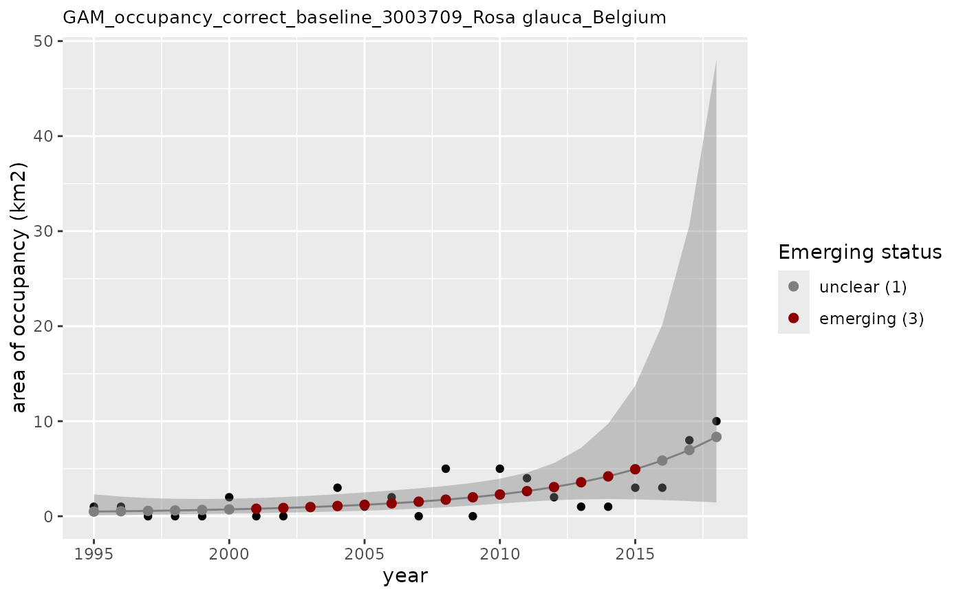
# How to use other arguments
apply_gam(df_gam,
y_var = "n",
eval_years = c(2017, 2018),
baseline_var = "n_class",
p_max = 0.3,
taxon_key = "3003709",
type_indicator = "occupancy",
name = "Rosa glauca",
df_title = "Belgium",
x_label = "time (years)",
y_label = "area of occupancy (km2)",
saveplot = TRUE,
dir_name = "./data/",
verbose = TRUE
)
#> width not provided. Set to 1680 pixels.
#> height not provided. Set to 1200 pixels.
#> [1] "Analyzing: Rosa glauca(3003709)"
#> [1] "Output plot: ./data/GAM_occupancy_correct_baseline_3003709_Rosa glauca_Belgium.png"
#> $em_summary
#> # A tibble: 2 × 5
#> taxonKey year em_status growth method
#> <dbl> <dbl> <dbl> <dbl> <chr>
#> 1 3003709 2017 1 0.989 correct_baseline
#> 2 3003709 2018 1 0.980 correct_baseline
#>
#> $model
#>
#> Family: Negative Binomial(2.907)
#> Link function: log
#>
#> Formula:
#> n ~ s(year, k = maxk, m = 3, bs = "tp") + s(n_class)
#>
#> Estimated degrees of freedom:
#> 2 1 total = 4
#>
#> REML score: 42.23685
#>
#> $output
#> # A tibble: 24 × 14
#> taxonKey canonicalName year n n_class method fit ucl lcl em1
#> <dbl> <chr> <dbl> <dbl> <dbl> <chr> <dbl> <dbl> <dbl> <dbl>
#> 1 3003709 Rosa glauca 1995 1 229 correct_b… 0.488 2.30 0.103 0
#> 2 3003709 Rosa glauca 1996 1 555 correct_b… 0.522 2.07 0.132 0
#> 3 3003709 Rosa glauca 1997 0 1116 correct_b… 0.561 1.92 0.164 0
#> 4 3003709 Rosa glauca 1998 0 939 correct_b… 0.606 1.84 0.200 0
#> 5 3003709 Rosa glauca 1999 0 919 correct_b… 0.658 1.82 0.239 0
#> 6 3003709 Rosa glauca 2000 2 853 correct_b… 0.719 1.84 0.280 0
#> 7 3003709 Rosa glauca 2001 0 442 correct_b… 0.789 1.91 0.325 0
#> 8 3003709 Rosa glauca 2002 0 532 correct_b… 0.870 2.02 0.375 1
#> 9 3003709 Rosa glauca 2003 1 623 correct_b… 0.964 2.16 0.431 1
#> 10 3003709 Rosa glauca 2004 3 1178 correct_b… 1.07 2.32 0.498 1
#> # ℹ 14 more rows
#> # ℹ 4 more variables: em2 <dbl>, em <dbl>, em_status <dbl>, growth <dbl>
#>
#> $first_derivative
#> # A tibble: 48 × 8
#> smooth derivative se crit lower_ci upper_ci year n_class
#> <chr> <dbl> <dbl> <dbl> <dbl> <dbl> <dbl> <dbl>
#> 1 s(year) 0.0647 0.131 1.28 -0.103 0.232 1995. NA
#> 2 s(year) 0.0698 0.120 1.28 -0.0840 0.224 1996. NA
#> 3 s(year) 0.0749 0.110 1.28 -0.0657 0.216 1997. NA
#> 4 s(year) 0.0800 0.0998 1.28 -0.0479 0.208 1998. NA
#> 5 s(year) 0.0851 0.0902 1.28 -0.0305 0.201 1999. NA
#> 6 s(year) 0.0902 0.0812 1.28 -0.0138 0.194 2000. NA
#> 7 s(year) 0.0953 0.0728 1.28 0.00198 0.189 2001. NA
#> 8 s(year) 0.100 0.0656 1.28 0.0164 0.184 2002. NA
#> 9 s(year) 0.106 0.0597 1.28 0.0291 0.182 2003. NA
#> 10 s(year) 0.111 0.0556 1.28 0.0394 0.182 2004. NA
#> # ℹ 38 more rows
#>
#> $second_derivative
#> # A tibble: 48 × 8
#> smooth derivative se crit lower_ci upper_ci year n_class
#> <chr> <dbl> <dbl> <dbl> <dbl> <dbl> <dbl> <dbl>
#> 1 s(year) 0.00511 0.0116 1.28 -0.00979 0.0200 1995. NA
#> 2 s(year) 0.00511 0.0116 1.28 -0.00979 0.0200 1996. NA
#> 3 s(year) 0.00511 0.0116 1.28 -0.00979 0.0200 1997. NA
#> 4 s(year) 0.00511 0.0116 1.28 -0.00979 0.0200 1998. NA
#> 5 s(year) 0.00511 0.0116 1.28 -0.00979 0.0200 1999. NA
#> 6 s(year) 0.00511 0.0116 1.28 -0.00979 0.0200 2000. NA
#> 7 s(year) 0.00511 0.0116 1.28 -0.00979 0.0200 2001. NA
#> 8 s(year) 0.00511 0.0116 1.28 -0.00979 0.0200 2002. NA
#> 9 s(year) 0.00511 0.0116 1.28 -0.00979 0.0200 2003. NA
#> 10 s(year) 0.00511 0.0116 1.28 -0.00979 0.0200 2004. NA
#> # ℹ 38 more rows
#>
#> $plot
#>
# How to use other arguments
apply_gam(df_gam,
y_var = "n",
eval_years = c(2017, 2018),
baseline_var = "n_class",
p_max = 0.3,
taxon_key = "3003709",
type_indicator = "occupancy",
name = "Rosa glauca",
df_title = "Belgium",
x_label = "time (years)",
y_label = "area of occupancy (km2)",
saveplot = TRUE,
dir_name = "./data/",
verbose = TRUE
)
#> width not provided. Set to 1680 pixels.
#> height not provided. Set to 1200 pixels.
#> [1] "Analyzing: Rosa glauca(3003709)"
#> [1] "Output plot: ./data/GAM_occupancy_correct_baseline_3003709_Rosa glauca_Belgium.png"
#> $em_summary
#> # A tibble: 2 × 5
#> taxonKey year em_status growth method
#> <dbl> <dbl> <dbl> <dbl> <chr>
#> 1 3003709 2017 1 0.989 correct_baseline
#> 2 3003709 2018 1 0.980 correct_baseline
#>
#> $model
#>
#> Family: Negative Binomial(2.907)
#> Link function: log
#>
#> Formula:
#> n ~ s(year, k = maxk, m = 3, bs = "tp") + s(n_class)
#>
#> Estimated degrees of freedom:
#> 2 1 total = 4
#>
#> REML score: 42.23685
#>
#> $output
#> # A tibble: 24 × 14
#> taxonKey canonicalName year n n_class method fit ucl lcl em1
#> <dbl> <chr> <dbl> <dbl> <dbl> <chr> <dbl> <dbl> <dbl> <dbl>
#> 1 3003709 Rosa glauca 1995 1 229 correct_b… 0.488 2.30 0.103 0
#> 2 3003709 Rosa glauca 1996 1 555 correct_b… 0.522 2.07 0.132 0
#> 3 3003709 Rosa glauca 1997 0 1116 correct_b… 0.561 1.92 0.164 0
#> 4 3003709 Rosa glauca 1998 0 939 correct_b… 0.606 1.84 0.200 0
#> 5 3003709 Rosa glauca 1999 0 919 correct_b… 0.658 1.82 0.239 0
#> 6 3003709 Rosa glauca 2000 2 853 correct_b… 0.719 1.84 0.280 0
#> 7 3003709 Rosa glauca 2001 0 442 correct_b… 0.789 1.91 0.325 0
#> 8 3003709 Rosa glauca 2002 0 532 correct_b… 0.870 2.02 0.375 1
#> 9 3003709 Rosa glauca 2003 1 623 correct_b… 0.964 2.16 0.431 1
#> 10 3003709 Rosa glauca 2004 3 1178 correct_b… 1.07 2.32 0.498 1
#> # ℹ 14 more rows
#> # ℹ 4 more variables: em2 <dbl>, em <dbl>, em_status <dbl>, growth <dbl>
#>
#> $first_derivative
#> # A tibble: 48 × 8
#> smooth derivative se crit lower_ci upper_ci year n_class
#> <chr> <dbl> <dbl> <dbl> <dbl> <dbl> <dbl> <dbl>
#> 1 s(year) 0.0647 0.131 1.28 -0.103 0.232 1995. NA
#> 2 s(year) 0.0698 0.120 1.28 -0.0840 0.224 1996. NA
#> 3 s(year) 0.0749 0.110 1.28 -0.0657 0.216 1997. NA
#> 4 s(year) 0.0800 0.0998 1.28 -0.0479 0.208 1998. NA
#> 5 s(year) 0.0851 0.0902 1.28 -0.0305 0.201 1999. NA
#> 6 s(year) 0.0902 0.0812 1.28 -0.0138 0.194 2000. NA
#> 7 s(year) 0.0953 0.0728 1.28 0.00198 0.189 2001. NA
#> 8 s(year) 0.100 0.0656 1.28 0.0164 0.184 2002. NA
#> 9 s(year) 0.106 0.0597 1.28 0.0291 0.182 2003. NA
#> 10 s(year) 0.111 0.0556 1.28 0.0394 0.182 2004. NA
#> # ℹ 38 more rows
#>
#> $second_derivative
#> # A tibble: 48 × 8
#> smooth derivative se crit lower_ci upper_ci year n_class
#> <chr> <dbl> <dbl> <dbl> <dbl> <dbl> <dbl> <dbl>
#> 1 s(year) 0.00511 0.0116 1.28 -0.00979 0.0200 1995. NA
#> 2 s(year) 0.00511 0.0116 1.28 -0.00979 0.0200 1996. NA
#> 3 s(year) 0.00511 0.0116 1.28 -0.00979 0.0200 1997. NA
#> 4 s(year) 0.00511 0.0116 1.28 -0.00979 0.0200 1998. NA
#> 5 s(year) 0.00511 0.0116 1.28 -0.00979 0.0200 1999. NA
#> 6 s(year) 0.00511 0.0116 1.28 -0.00979 0.0200 2000. NA
#> 7 s(year) 0.00511 0.0116 1.28 -0.00979 0.0200 2001. NA
#> 8 s(year) 0.00511 0.0116 1.28 -0.00979 0.0200 2002. NA
#> 9 s(year) 0.00511 0.0116 1.28 -0.00979 0.0200 2003. NA
#> 10 s(year) 0.00511 0.0116 1.28 -0.00979 0.0200 2004. NA
#> # ℹ 38 more rows
#>
#> $plot
 #>
# warning returned if GAM cannot be applied and plot with only observations
df_gam <- tibble(
taxonKey = rep(3003709, 24),
canonicalName = rep("Rosa glauca", 24),
year = seq(1995, 2018),
obs = c(
1, 1, 0, 0, 0, 2, 0, 0, 1, 3, 1, 2, 0, 5, 0, 5, 4, 2, 1,
1, 3, 3, 8, 10
),
cobs = rep(0, 24)
)
# if GAM cannot be applied a warning is returned and the plot mention it by default.
if (FALSE) { # \dontrun{
# With textual annotation in the plot
no_gam_with_annotation <- apply_gam(
df_gam[19:24,],
y_var = "n",
eval_years = 2018,
taxon_key = 3003709,
name = "Rosa glauca",
baseline_var = "n_class",
verbose = TRUE
)
no_gam_with_annotation$plot
# Without textual annotation in the plot
no_gam_without_annotation <- apply_gam(
df_gam[19:24,],
y_var = "n",
eval_years = 2018,
taxon_key = 3003709,
name = "Rosa glauca",
baseline_var = "n_class",
verbose = TRUE,
status_warning = FALSE
)
no_gam_without_annotation$plot
} # }
#>
# warning returned if GAM cannot be applied and plot with only observations
df_gam <- tibble(
taxonKey = rep(3003709, 24),
canonicalName = rep("Rosa glauca", 24),
year = seq(1995, 2018),
obs = c(
1, 1, 0, 0, 0, 2, 0, 0, 1, 3, 1, 2, 0, 5, 0, 5, 4, 2, 1,
1, 3, 3, 8, 10
),
cobs = rep(0, 24)
)
# if GAM cannot be applied a warning is returned and the plot mention it by default.
if (FALSE) { # \dontrun{
# With textual annotation in the plot
no_gam_with_annotation <- apply_gam(
df_gam[19:24,],
y_var = "n",
eval_years = 2018,
taxon_key = 3003709,
name = "Rosa glauca",
baseline_var = "n_class",
verbose = TRUE
)
no_gam_with_annotation$plot
# Without textual annotation in the plot
no_gam_without_annotation <- apply_gam(
df_gam[19:24,],
y_var = "n",
eval_years = 2018,
taxon_key = 3003709,
name = "Rosa glauca",
baseline_var = "n_class",
verbose = TRUE,
status_warning = FALSE
)
no_gam_without_annotation$plot
} # }